In this work we used dispersion of regional surface waves (Rayleigh wave group velocity) to constrain shear-wave velocity as a function of depth at ten locations in the Ladakh region of the NW Himalaya. Details are in our 2009 Tectonophysics paper (citation information at the bottom of this page). We used regional earthquakes (~300-900 km distant) recorded on an array of 16 stations run by India's National Geophysical Research Institute (NGRI) and Cambridge University.
Our inversions used Robert Herrmann's Computer Programs in Seismology.
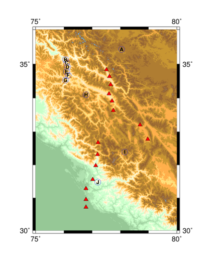
The velocity profiles are in tab-delimited text files, one for each of the 10 regions over which we grouped and averaged dispersion curves and derived a mean velocity model (see Section 2.3 in the paper). Each filename suffix (A through J) in the archive corresponds to one of these regions (see Figure 1b and Figure 3 in the paper).
The files in the archive have the following column structure:
*Our inversion was for S-velocity; P-velocity is calculated from S-velocity using a fixed Vp/Vs ratio of 1.76.
Each dispersion curve represents average velocities for the earthquake-to-station path, and each of our ten regions average many dispersion curves, and thus there is no single lat/lon location at which to locate each profile. However, the following table gives the mean location of the midpoints of the earthquake-station paths used to calculate each profile, and is thus the best single location to associate with the profiles.
| A | 35.431 | 78.046 |
| B | 35.133 | 76.055 |
| C | 35.044 | 76.099 |
| D | 34.913 | 76.129 |
| E | 34.775 | 76.095 |
| F | 34.668 | 76.149 |
| G | 34.533 | 76.056 |
| H | 34.104 | 76.786 |
| I | 32.394 | 78.157 |
| J | 31.482 | 77.203 |
This table is also in the data archive as Midpoints.xy.
CLICK HERE TO DOWNLOAD DATA ARCHIVE
This map shows the location of the mean midpoint for each of the ten regions. GMT code included in archive as MakeMap.gmt, as well a postscript version of the map as MidpointLocations.ps.

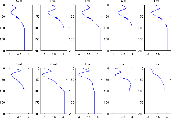
This plot is a simplified version of Figure 3 from the paper. A MATLAB script for generating this figure is in the data archive as PlotVelocities.m.

A word about depth: These plots extend to 200 km depth because the last row of each velocity file is listed as 100-200 km depth, but this row actually represents a half-space below 100 km. In reality, because our dispersion curves did not extend past 50 seconds period, the models are only reliable down to 75 km depth.
W.B. Caldwell, S.L. Klemperer, S.S. Rai, and J.F. Lawrence, Partial melt in the upper-middle crust of the northwest Himalaya revealed by Rayleigh wave dispersion, Tectonophysics, Vol. 477, Iss. 1-2, Pages 58-65, 1 November 2009, doi:10.1016/j.tecto.2009.01.013.